AI/Intermediate
00_intro_sklearn
해쨔니
2022. 7. 25. 21:06

Scikit-Learn
In [ ]:
import matplotlib.pyplot as plt
import numpy as np
import pandas as pd
특징
- 가장 유명한 머신러닝 알고리즘
- 다양한 머신러닝 알고리즘을 효율적으로 구현하여 제공
- 서로 다른 알고리즘에 동일한 인터페이스 제공
- numpy, padas등 다른 라이브러리와 높은 호환성
- 알고리즘은 Classifier와 Regressor로 구성됨
입력
특징 행렬
- 알고리즘의 입력으로 주로 변수명을 X_train, X_test로 코딩하고 항상 (N,D)가 되는 행렬
대상 배열
- 지도 학습에서 알고리즘의 예측 대상으로 주로 y_train, y_test로 코딩하고 항상 (N,)인 벡터
In [ ]:
# source: https://jakevdp.github.io/PythonDataScienceHandbook/06.00-figure-code.html#Features-and-Labels-Grid

fig = plt.figure(figsize=(6, 4))
ax = fig.add_axes([0, 0, 1, 1])
ax.axis('off')
ax.axis('equal')

# Draw features matrix
ax.vlines(range(6), ymin=0, ymax=9, lw=1)
ax.hlines(range(10), xmin=0, xmax=5, lw=1)
font_prop = dict(size=12, family='monospace')
ax.text(-1, -1, "Feature Matrix ($X$)", size=14)
ax.text(0.1, -0.3, r'n_features $\longrightarrow$', **font_prop)
ax.text(-0.1, 0.1, r'$\longleftarrow$ n_samples', rotation=90,
        va='top', ha='right', **font_prop)

# Draw labels vector
ax.vlines(range(8, 10), ymin=0, ymax=9, lw=1)
ax.hlines(range(10), xmin=8, xmax=9, lw=1)
ax.text(7, -1, "Target Vector ($y$)", size=14)
ax.text(7.9, 0.1, r'$\longleftarrow$ n_samples', rotation=90,
        va='top', ha='right', **font_prop)

ax.set_ylim(10, -2)

plt.show()

API 표준 사용법
- 적절한 추정기(알고리즘)을 임포트 한다.
- 임포트한 추정기를 객체로 만든다. 이때 각 알고리즘이 요구하는 초모수hyper parameters를 선택한다.
- 데이터를 '입력'에서 이야기한 방식으로 맞춘다.
- fit(X, y)해서 모델을 데이터에 피팅한다.
- 모델을 새 데이터에 적용한다.
- predict(): 모델 예측값을 출력
- predict_proba(): 모델 예측의 확률을 출력
- transform(): 입력을 적절한 형태로 변환, 예) 단어를 벡터로 변환
predict(), predict_proba()
In [ ]:
from sklearn import tree

X_train = [[0, 0], [1, 1]]
y_train = [0, 1]

######################################
# 결정트리 생성과 fit[+]
clf = tree.DecisionTreeClassifier()
clf = clf.fit(X_train, y_train)
In [ ]:
#########################
# 예측[+]
clf.predict([[2., 2.]])
# 타겟 예측
clf.predict([[0,1]])

# 확률로 예측
clf.predict_proba([[0,1]])
Out[ ]:
array([[1., 0.]])transform()
In [ ]:
# 스케일러 transform 하는것
# 데이터의 최대값과 최소값을 사용해 0~1로 점위를 수정

# 모델로딩
from sklearn.preprocessing import MinMaxScaler
In [ ]:
X_train = np.array([[0.1, 0.8, 0.4, 0.2, 0.9], [1.1, 10.9, 4.5, 2.3, 7.1]]).T

fig = plt.figure(dpi=100)
ax = plt.axes()

ax.plot(X_train[:,0], X_train[:,1], 'o', color='C1')
ax.axis('equal')

plt.show()

print(X_train)

[[ 0.1  1.1]
 [ 0.8 10.9]
 [ 0.4  4.5]
 [ 0.2  2.3]
 [ 0.9  7.1]]
In [ ]:
# 모델 생성과 fit[+]
scaler = MinMaxScaler()
scaler.fit(X_train)
print(scaler.data_max_, scaler.data_min_) # 각 column마다 추출
[ 0.9 10.9] [0.1 1.1]
In [ ]:
# transform[+]
X_train_scaled = scaler.transform(X_train)

fig = plt.figure(dpi=100)
ax = plt.axes()

ax.plot(X_train_scaled[:,0], X_train_scaled[:,1], 'o', color='C1')
ax.axis('equal')

plt.show()

print(X_train_scaled)

[[0.         0.        ]
 [0.875      1.        ]
 [0.375      0.34693878]
 [0.125      0.12244898]
 [1.         0.6122449 ]]
제공되는 기본 데이터
Iris
In [ ]:
# 데이터 로딩[+]
from sklearn.datasets import load_iris

iris = load_iris()
In [ ]:
# description[+]
print(iris.DESCR)
.. _iris_dataset:

Iris plants dataset
--------------------

**Data Set Characteristics:**

    :Number of Instances: 150 (50 in each of three classes)
    :Number of Attributes: 4 numeric, predictive attributes and the class
    :Attribute Information:
        - sepal length in cm
        - sepal width in cm
        - petal length in cm
        - petal width in cm
        - class:
                - Iris-Setosa
                - Iris-Versicolour
                - Iris-Virginica

    :Summary Statistics:

    ============== ==== ==== ======= ===== ====================
                    Min  Max   Mean    SD   Class Correlation
    ============== ==== ==== ======= ===== ====================
    sepal length:   4.3  7.9   5.84   0.83    0.7826
    sepal width:    2.0  4.4   3.05   0.43   -0.4194
    petal length:   1.0  6.9   3.76   1.76    0.9490  (high!)
    petal width:    0.1  2.5   1.20   0.76    0.9565  (high!)
    ============== ==== ==== ======= ===== ====================

    :Missing Attribute Values: None
    :Class Distribution: 33.3% for each of 3 classes.
    :Creator: R.A. Fisher
    :Donor: Michael Marshall (MARSHALL%PLU@io.arc.nasa.gov)
    :Date: July, 1988

The famous Iris database, first used by Sir R.A. Fisher. The dataset is taken
from Fisher's paper. Note that it's the same as in R, but not as in the UCI
Machine Learning Repository, which has two wrong data points.

This is perhaps the best known database to be found in the
pattern recognition literature.  Fisher's paper is a classic in the field and
is referenced frequently to this day.  (See Duda & Hart, for example.)  The
data set contains 3 classes of 50 instances each, where each class refers to a
type of iris plant.  One class is linearly separable from the other 2; the
latter are NOT linearly separable from each other.

.. topic:: References

   - Fisher, R.A. "The use of multiple measurements in taxonomic problems"
     Annual Eugenics, 7, Part II, 179-188 (1936); also in "Contributions to
     Mathematical Statistics" (John Wiley, NY, 1950).
   - Duda, R.O., & Hart, P.E. (1973) Pattern Classification and Scene Analysis.
     (Q327.D83) John Wiley & Sons.  ISBN 0-471-22361-1.  See page 218.
   - Dasarathy, B.V. (1980) "Nosing Around the Neighborhood: A New System
     Structure and Classification Rule for Recognition in Partially Exposed
     Environments".  IEEE Transactions on Pattern Analysis and Machine
     Intelligence, Vol. PAMI-2, No. 1, 67-71.
   - Gates, G.W. (1972) "The Reduced Nearest Neighbor Rule".  IEEE Transactions
     on Information Theory, May 1972, 431-433.
   - See also: 1988 MLC Proceedings, 54-64.  Cheeseman et al"s AUTOCLASS II
     conceptual clustering system finds 3 classes in the data.
   - Many, many more ...
In [ ]:
# 데이터 확인[+]
print(type(iris.data))
iris.data[:10]
<class 'numpy.ndarray'>
Out[ ]:
array([[5.1, 3.5, 1.4, 0.2],
       [4.9, 3. , 1.4, 0.2],
       [4.7, 3.2, 1.3, 0.2],
       [4.6, 3.1, 1.5, 0.2],
       [5. , 3.6, 1.4, 0.2],
       [5.4, 3.9, 1.7, 0.4],
       [4.6, 3.4, 1.4, 0.3],
       [5. , 3.4, 1.5, 0.2],
       [4.4, 2.9, 1.4, 0.2],
       [4.9, 3.1, 1.5, 0.1]])
In [ ]:
# 타겟 확인[+]
iris.target
Out[ ]:
array([0, 0, 0, 0, 0, 0, 0, 0, 0, 0, 0, 0, 0, 0, 0, 0, 0, 0, 0, 0, 0, 0,
       0, 0, 0, 0, 0, 0, 0, 0, 0, 0, 0, 0, 0, 0, 0, 0, 0, 0, 0, 0, 0, 0,
       0, 0, 0, 0, 0, 0, 1, 1, 1, 1, 1, 1, 1, 1, 1, 1, 1, 1, 1, 1, 1, 1,
       1, 1, 1, 1, 1, 1, 1, 1, 1, 1, 1, 1, 1, 1, 1, 1, 1, 1, 1, 1, 1, 1,
       1, 1, 1, 1, 1, 1, 1, 1, 1, 1, 1, 1, 2, 2, 2, 2, 2, 2, 2, 2, 2, 2,
       2, 2, 2, 2, 2, 2, 2, 2, 2, 2, 2, 2, 2, 2, 2, 2, 2, 2, 2, 2, 2, 2,
       2, 2, 2, 2, 2, 2, 2, 2, 2, 2, 2, 2, 2, 2, 2, 2, 2, 2])
Breast Cancer
In [ ]:
# 데이터 로딩[+]
from sklearn.datasets import load_breast_cancer
breast_cancer = load_breast_cancer()
In [ ]:
# description[+]

print(breast_cancer.DESCR)
.. _breast_cancer_dataset:

Breast cancer wisconsin (diagnostic) dataset
--------------------------------------------

**Data Set Characteristics:**

    :Number of Instances: 569

    :Number of Attributes: 30 numeric, predictive attributes and the class

    :Attribute Information:
        - radius (mean of distances from center to points on the perimeter)
        - texture (standard deviation of gray-scale values)
        - perimeter
        - area
        - smoothness (local variation in radius lengths)
        - compactness (perimeter^2 / area - 1.0)
        - concavity (severity of concave portions of the contour)
        - concave points (number of concave portions of the contour)
        - symmetry
        - fractal dimension ("coastline approximation" - 1)

        The mean, standard error, and "worst" or largest (mean of the three
        worst/largest values) of these features were computed for each image,
        resulting in 30 features.  For instance, field 0 is Mean Radius, field
        10 is Radius SE, field 20 is Worst Radius.

        - class:
                - WDBC-Malignant
                - WDBC-Benign

    :Summary Statistics:

    ===================================== ====== ======
                                           Min    Max
    ===================================== ====== ======
    radius (mean):                        6.981  28.11
    texture (mean):                       9.71   39.28
    perimeter (mean):                     43.79  188.5
    area (mean):                          143.5  2501.0
    smoothness (mean):                    0.053  0.163
    compactness (mean):                   0.019  0.345
    concavity (mean):                     0.0    0.427
    concave points (mean):                0.0    0.201
    symmetry (mean):                      0.106  0.304
    fractal dimension (mean):             0.05   0.097
    radius (standard error):              0.112  2.873
    texture (standard error):             0.36   4.885
    perimeter (standard error):           0.757  21.98
    area (standard error):                6.802  542.2
    smoothness (standard error):          0.002  0.031
    compactness (standard error):         0.002  0.135
    concavity (standard error):           0.0    0.396
    concave points (standard error):      0.0    0.053
    symmetry (standard error):            0.008  0.079
    fractal dimension (standard error):   0.001  0.03
    radius (worst):                       7.93   36.04
    texture (worst):                      12.02  49.54
    perimeter (worst):                    50.41  251.2
    area (worst):                         185.2  4254.0
    smoothness (worst):                   0.071  0.223
    compactness (worst):                  0.027  1.058
    concavity (worst):                    0.0    1.252
    concave points (worst):               0.0    0.291
    symmetry (worst):                     0.156  0.664
    fractal dimension (worst):            0.055  0.208
    ===================================== ====== ======

    :Missing Attribute Values: None

    :Class Distribution: 212 - Malignant, 357 - Benign

    :Creator:  Dr. William H. Wolberg, W. Nick Street, Olvi L. Mangasarian

    :Donor: Nick Street

    :Date: November, 1995

This is a copy of UCI ML Breast Cancer Wisconsin (Diagnostic) datasets.
https://goo.gl/U2Uwz2

Features are computed from a digitized image of a fine needle
aspirate (FNA) of a breast mass.  They describe
characteristics of the cell nuclei present in the image.

Separating plane described above was obtained using
Multisurface Method-Tree (MSM-T) [K. P. Bennett, "Decision Tree
Construction Via Linear Programming." Proceedings of the 4th
Midwest Artificial Intelligence and Cognitive Science Society,
pp. 97-101, 1992], a classification method which uses linear
programming to construct a decision tree.  Relevant features
were selected using an exhaustive search in the space of 1-4
features and 1-3 separating planes.

The actual linear program used to obtain the separating plane
in the 3-dimensional space is that described in:
[K. P. Bennett and O. L. Mangasarian: "Robust Linear
Programming Discrimination of Two Linearly Inseparable Sets",
Optimization Methods and Software 1, 1992, 23-34].

This database is also available through the UW CS ftp server:

ftp ftp.cs.wisc.edu
cd math-prog/cpo-dataset/machine-learn/WDBC/

.. topic:: References

   - W.N. Street, W.H. Wolberg and O.L. Mangasarian. Nuclear feature extraction
     for breast tumor diagnosis. IS&T/SPIE 1993 International Symposium on
     Electronic Imaging: Science and Technology, volume 1905, pages 861-870,
     San Jose, CA, 1993.
   - O.L. Mangasarian, W.N. Street and W.H. Wolberg. Breast cancer diagnosis and
     prognosis via linear programming. Operations Research, 43(4), pages 570-577,
     July-August 1995.
   - W.H. Wolberg, W.N. Street, and O.L. Mangasarian. Machine learning techniques
     to diagnose breast cancer from fine-needle aspirates. Cancer Letters 77 (1994)
     163-171.
In [ ]:
# 데이터 확인[+]
'''df = pd.DataFrame(breast_cancer.data, columns=breast_cancer.feature_names)
sy = pd.Series(breast_cancer.target, dtype="category")
sy = sy.cat.rename_categories(breast_cancer.target_names)
df['class'] = sy
df.tail()'''

breast_cancer.data[:5]
Out[ ]:
array([[1.799e+01, 1.038e+01, 1.228e+02, 1.001e+03, 1.184e-01, 2.776e-01,
        3.001e-01, 1.471e-01, 2.419e-01, 7.871e-02, 1.095e+00, 9.053e-01,
        8.589e+00, 1.534e+02, 6.399e-03, 4.904e-02, 5.373e-02, 1.587e-02,
        3.003e-02, 6.193e-03, 2.538e+01, 1.733e+01, 1.846e+02, 2.019e+03,
        1.622e-01, 6.656e-01, 7.119e-01, 2.654e-01, 4.601e-01, 1.189e-01],
       [2.057e+01, 1.777e+01, 1.329e+02, 1.326e+03, 8.474e-02, 7.864e-02,
        8.690e-02, 7.017e-02, 1.812e-01, 5.667e-02, 5.435e-01, 7.339e-01,
        3.398e+00, 7.408e+01, 5.225e-03, 1.308e-02, 1.860e-02, 1.340e-02,
        1.389e-02, 3.532e-03, 2.499e+01, 2.341e+01, 1.588e+02, 1.956e+03,
        1.238e-01, 1.866e-01, 2.416e-01, 1.860e-01, 2.750e-01, 8.902e-02],
       [1.969e+01, 2.125e+01, 1.300e+02, 1.203e+03, 1.096e-01, 1.599e-01,
        1.974e-01, 1.279e-01, 2.069e-01, 5.999e-02, 7.456e-01, 7.869e-01,
        4.585e+00, 9.403e+01, 6.150e-03, 4.006e-02, 3.832e-02, 2.058e-02,
        2.250e-02, 4.571e-03, 2.357e+01, 2.553e+01, 1.525e+02, 1.709e+03,
        1.444e-01, 4.245e-01, 4.504e-01, 2.430e-01, 3.613e-01, 8.758e-02],
       [1.142e+01, 2.038e+01, 7.758e+01, 3.861e+02, 1.425e-01, 2.839e-01,
        2.414e-01, 1.052e-01, 2.597e-01, 9.744e-02, 4.956e-01, 1.156e+00,
        3.445e+00, 2.723e+01, 9.110e-03, 7.458e-02, 5.661e-02, 1.867e-02,
        5.963e-02, 9.208e-03, 1.491e+01, 2.650e+01, 9.887e+01, 5.677e+02,
        2.098e-01, 8.663e-01, 6.869e-01, 2.575e-01, 6.638e-01, 1.730e-01],
       [2.029e+01, 1.434e+01, 1.351e+02, 1.297e+03, 1.003e-01, 1.328e-01,
        1.980e-01, 1.043e-01, 1.809e-01, 5.883e-02, 7.572e-01, 7.813e-01,
        5.438e+00, 9.444e+01, 1.149e-02, 2.461e-02, 5.688e-02, 1.885e-02,
        1.756e-02, 5.115e-03, 2.254e+01, 1.667e+01, 1.522e+02, 1.575e+03,
        1.374e-01, 2.050e-01, 4.000e-01, 1.625e-01, 2.364e-01, 7.678e-02]])
In [ ]:
# 타겟 확인[+]
print(breast_cancer.target)
breast_cancer.target_names
[0 0 0 0 0 0 0 0 0 0 0 0 0 0 0 0 0 0 0 1 1 1 0 0 0 0 0 0 0 0 0 0 0 0 0 0 0
 1 0 0 0 0 0 0 0 0 1 0 1 1 1 1 1 0 0 1 0 0 1 1 1 1 0 1 0 0 1 1 1 1 0 1 0 0
 1 0 1 0 0 1 1 1 0 0 1 0 0 0 1 1 1 0 1 1 0 0 1 1 1 0 0 1 1 1 1 0 1 1 0 1 1
 1 1 1 1 1 1 0 0 0 1 0 0 1 1 1 0 0 1 0 1 0 0 1 0 0 1 1 0 1 1 0 1 1 1 1 0 1
 1 1 1 1 1 1 1 1 0 1 1 1 1 0 0 1 0 1 1 0 0 1 1 0 0 1 1 1 1 0 1 1 0 0 0 1 0
 1 0 1 1 1 0 1 1 0 0 1 0 0 0 0 1 0 0 0 1 0 1 0 1 1 0 1 0 0 0 0 1 1 0 0 1 1
 1 0 1 1 1 1 1 0 0 1 1 0 1 1 0 0 1 0 1 1 1 1 0 1 1 1 1 1 0 1 0 0 0 0 0 0 0
 0 0 0 0 0 0 0 1 1 1 1 1 1 0 1 0 1 1 0 1 1 0 1 0 0 1 1 1 1 1 1 1 1 1 1 1 1
 1 0 1 1 0 1 0 1 1 1 1 1 1 1 1 1 1 1 1 1 1 0 1 1 1 0 1 0 1 1 1 1 0 0 0 1 1
 1 1 0 1 0 1 0 1 1 1 0 1 1 1 1 1 1 1 0 0 0 1 1 1 1 1 1 1 1 1 1 1 0 0 1 0 0
 0 1 0 0 1 1 1 1 1 0 1 1 1 1 1 0 1 1 1 0 1 1 0 0 1 1 1 1 1 1 0 1 1 1 1 1 1
 1 0 1 1 1 1 1 0 1 1 0 1 1 1 1 1 1 1 1 1 1 1 1 0 1 0 0 1 0 1 1 1 1 1 0 1 1
 0 1 0 1 1 0 1 0 1 1 1 1 1 1 1 1 0 0 1 1 1 1 1 1 0 1 1 1 1 1 1 1 1 1 1 0 1
 1 1 1 1 1 1 0 1 0 1 1 0 1 1 1 1 1 0 0 1 0 1 0 1 1 1 1 1 0 1 1 0 1 0 1 0 0
 1 1 1 0 1 1 1 1 1 1 1 1 1 1 1 0 1 0 0 1 1 1 1 1 1 1 1 1 1 1 1 1 1 1 1 1 1
 1 1 1 1 1 1 1 0 0 0 0 0 0 1]
Out[ ]:
array(['malignant', 'benign'], dtype='<U9')Boston House Price
In [ ]:
# 데이터 로딩[+]
from sklearn.datasets import load_boston
boston = load_boston()
/usr/local/lib/python3.7/dist-packages/sklearn/utils/deprecation.py:87: FutureWarning: Function load_boston is deprecated; `load_boston` is deprecated in 1.0 and will be removed in 1.2.

    The Boston housing prices dataset has an ethical problem. You can refer to
    the documentation of this function for further details.

    The scikit-learn maintainers therefore strongly discourage the use of this
    dataset unless the purpose of the code is to study and educate about
    ethical issues in data science and machine learning.

    In this special case, you can fetch the dataset from the original
    source::

        import pandas as pd
        import numpy as np


        data_url = "http://lib.stat.cmu.edu/datasets/boston"
        raw_df = pd.read_csv(data_url, sep="\s+", skiprows=22, header=None)
        data = np.hstack([raw_df.values[::2, :], raw_df.values[1::2, :2]])
        target = raw_df.values[1::2, 2]

    Alternative datasets include the California housing dataset (i.e.
    :func:`~sklearn.datasets.fetch_california_housing`) and the Ames housing
    dataset. You can load the datasets as follows::

        from sklearn.datasets import fetch_california_housing
        housing = fetch_california_housing()

    for the California housing dataset and::

        from sklearn.datasets import fetch_openml
        housing = fetch_openml(name="house_prices", as_frame=True)

    for the Ames housing dataset.

  warnings.warn(msg, category=FutureWarning)
In [ ]:
# description[+]
print(boston.DESCR)
.. _boston_dataset:

Boston house prices dataset
---------------------------

**Data Set Characteristics:**

    :Number of Instances: 506

    :Number of Attributes: 13 numeric/categorical predictive. Median Value (attribute 14) is usually the target.

    :Attribute Information (in order):
        - CRIM     per capita crime rate by town
        - ZN       proportion of residential land zoned for lots over 25,000 sq.ft.
        - INDUS    proportion of non-retail business acres per town
        - CHAS     Charles River dummy variable (= 1 if tract bounds river; 0 otherwise)
        - NOX      nitric oxides concentration (parts per 10 million)
        - RM       average number of rooms per dwelling
        - AGE      proportion of owner-occupied units built prior to 1940
        - DIS      weighted distances to five Boston employment centres
        - RAD      index of accessibility to radial highways
        - TAX      full-value property-tax rate per $10,000
        - PTRATIO  pupil-teacher ratio by town
        - B        1000(Bk - 0.63)^2 where Bk is the proportion of black people by town
        - LSTAT    % lower status of the population
        - MEDV     Median value of owner-occupied homes in $1000's

    :Missing Attribute Values: None

    :Creator: Harrison, D. and Rubinfeld, D.L.

This is a copy of UCI ML housing dataset.
https://archive.ics.uci.edu/ml/machine-learning-databases/housing/


This dataset was taken from the StatLib library which is maintained at Carnegie Mellon University.

The Boston house-price data of Harrison, D. and Rubinfeld, D.L. 'Hedonic
prices and the demand for clean air', J. Environ. Economics & Management,
vol.5, 81-102, 1978.   Used in Belsley, Kuh & Welsch, 'Regression diagnostics
...', Wiley, 1980.   N.B. Various transformations are used in the table on
pages 244-261 of the latter.

The Boston house-price data has been used in many machine learning papers that address regression
problems.

.. topic:: References

   - Belsley, Kuh & Welsch, 'Regression diagnostics: Identifying Influential Data and Sources of Collinearity', Wiley, 1980. 244-261.
   - Quinlan,R. (1993). Combining Instance-Based and Model-Based Learning. In Proceedings on the Tenth International Conference of Machine Learning, 236-243, University of Massachusetts, Amherst. Morgan Kaufmann.
In [ ]:
# 데이터 확인[+]
print(boston.data[:2])


dfX = pd.DataFrame(boston.data, columns=boston.feature_names)
dfy = pd.DataFrame(boston.target, columns=["MEDV"])
df_house = pd.concat([dfX, dfy], axis=1)
df_house.tail(10)
[[6.3200e-03 1.8000e+01 2.3100e+00 0.0000e+00 5.3800e-01 6.5750e+00
  6.5200e+01 4.0900e+00 1.0000e+00 2.9600e+02 1.5300e+01 3.9690e+02
  4.9800e+00]
 [2.7310e-02 0.0000e+00 7.0700e+00 0.0000e+00 4.6900e-01 6.4210e+00
  7.8900e+01 4.9671e+00 2.0000e+00 2.4200e+02 1.7800e+01 3.9690e+02
  9.1400e+00]]
Out[ ]:
CRIMZNINDUSCHASNOXRMAGEDISRADTAXPTRATIOBLSTATMEDV496497498499500501502503504505
| 0.28960 | 0.0 | 9.69 | 0.0 | 0.585 | 5.390 | 72.9 | 2.7986 | 6.0 | 391.0 | 19.2 | 396.90 | 21.14 | 19.7 |
| 0.26838 | 0.0 | 9.69 | 0.0 | 0.585 | 5.794 | 70.6 | 2.8927 | 6.0 | 391.0 | 19.2 | 396.90 | 14.10 | 18.3 |
| 0.23912 | 0.0 | 9.69 | 0.0 | 0.585 | 6.019 | 65.3 | 2.4091 | 6.0 | 391.0 | 19.2 | 396.90 | 12.92 | 21.2 |
| 0.17783 | 0.0 | 9.69 | 0.0 | 0.585 | 5.569 | 73.5 | 2.3999 | 6.0 | 391.0 | 19.2 | 395.77 | 15.10 | 17.5 |
| 0.22438 | 0.0 | 9.69 | 0.0 | 0.585 | 6.027 | 79.7 | 2.4982 | 6.0 | 391.0 | 19.2 | 396.90 | 14.33 | 16.8 |
| 0.06263 | 0.0 | 11.93 | 0.0 | 0.573 | 6.593 | 69.1 | 2.4786 | 1.0 | 273.0 | 21.0 | 391.99 | 9.67 | 22.4 |
| 0.04527 | 0.0 | 11.93 | 0.0 | 0.573 | 6.120 | 76.7 | 2.2875 | 1.0 | 273.0 | 21.0 | 396.90 | 9.08 | 20.6 |
| 0.06076 | 0.0 | 11.93 | 0.0 | 0.573 | 6.976 | 91.0 | 2.1675 | 1.0 | 273.0 | 21.0 | 396.90 | 5.64 | 23.9 |
| 0.10959 | 0.0 | 11.93 | 0.0 | 0.573 | 6.794 | 89.3 | 2.3889 | 1.0 | 273.0 | 21.0 | 393.45 | 6.48 | 22.0 |
| 0.04741 | 0.0 | 11.93 | 0.0 | 0.573 | 6.030 | 80.8 | 2.5050 | 1.0 | 273.0 | 21.0 | 396.90 | 7.88 | 11.9 |
In [ ]:
# 타겟 확인[+]
boston.target
Out[ ]:
array([24. , 21.6, 34.7, 33.4, 36.2, 28.7, 22.9, 27.1, 16.5, 18.9, 15. ,
       18.9, 21.7, 20.4, 18.2, 19.9, 23.1, 17.5, 20.2, 18.2, 13.6, 19.6,
       15.2, 14.5, 15.6, 13.9, 16.6, 14.8, 18.4, 21. , 12.7, 14.5, 13.2,
       13.1, 13.5, 18.9, 20. , 21. , 24.7, 30.8, 34.9, 26.6, 25.3, 24.7,
       21.2, 19.3, 20. , 16.6, 14.4, 19.4, 19.7, 20.5, 25. , 23.4, 18.9,
       35.4, 24.7, 31.6, 23.3, 19.6, 18.7, 16. , 22.2, 25. , 33. , 23.5,
       19.4, 22. , 17.4, 20.9, 24.2, 21.7, 22.8, 23.4, 24.1, 21.4, 20. ,
       20.8, 21.2, 20.3, 28. , 23.9, 24.8, 22.9, 23.9, 26.6, 22.5, 22.2,
       23.6, 28.7, 22.6, 22. , 22.9, 25. , 20.6, 28.4, 21.4, 38.7, 43.8,
       33.2, 27.5, 26.5, 18.6, 19.3, 20.1, 19.5, 19.5, 20.4, 19.8, 19.4,
       21.7, 22.8, 18.8, 18.7, 18.5, 18.3, 21.2, 19.2, 20.4, 19.3, 22. ,
       20.3, 20.5, 17.3, 18.8, 21.4, 15.7, 16.2, 18. , 14.3, 19.2, 19.6,
       23. , 18.4, 15.6, 18.1, 17.4, 17.1, 13.3, 17.8, 14. , 14.4, 13.4,
       15.6, 11.8, 13.8, 15.6, 14.6, 17.8, 15.4, 21.5, 19.6, 15.3, 19.4,
       17. , 15.6, 13.1, 41.3, 24.3, 23.3, 27. , 50. , 50. , 50. , 22.7,
       25. , 50. , 23.8, 23.8, 22.3, 17.4, 19.1, 23.1, 23.6, 22.6, 29.4,
       23.2, 24.6, 29.9, 37.2, 39.8, 36.2, 37.9, 32.5, 26.4, 29.6, 50. ,
       32. , 29.8, 34.9, 37. , 30.5, 36.4, 31.1, 29.1, 50. , 33.3, 30.3,
       34.6, 34.9, 32.9, 24.1, 42.3, 48.5, 50. , 22.6, 24.4, 22.5, 24.4,
       20. , 21.7, 19.3, 22.4, 28.1, 23.7, 25. , 23.3, 28.7, 21.5, 23. ,
       26.7, 21.7, 27.5, 30.1, 44.8, 50. , 37.6, 31.6, 46.7, 31.5, 24.3,
       31.7, 41.7, 48.3, 29. , 24. , 25.1, 31.5, 23.7, 23.3, 22. , 20.1,
       22.2, 23.7, 17.6, 18.5, 24.3, 20.5, 24.5, 26.2, 24.4, 24.8, 29.6,
       42.8, 21.9, 20.9, 44. , 50. , 36. , 30.1, 33.8, 43.1, 48.8, 31. ,
       36.5, 22.8, 30.7, 50. , 43.5, 20.7, 21.1, 25.2, 24.4, 35.2, 32.4,
       32. , 33.2, 33.1, 29.1, 35.1, 45.4, 35.4, 46. , 50. , 32.2, 22. ,
       20.1, 23.2, 22.3, 24.8, 28.5, 37.3, 27.9, 23.9, 21.7, 28.6, 27.1,
       20.3, 22.5, 29. , 24.8, 22. , 26.4, 33.1, 36.1, 28.4, 33.4, 28.2,
       22.8, 20.3, 16.1, 22.1, 19.4, 21.6, 23.8, 16.2, 17.8, 19.8, 23.1,
       21. , 23.8, 23.1, 20.4, 18.5, 25. , 24.6, 23. , 22.2, 19.3, 22.6,
       19.8, 17.1, 19.4, 22.2, 20.7, 21.1, 19.5, 18.5, 20.6, 19. , 18.7,
       32.7, 16.5, 23.9, 31.2, 17.5, 17.2, 23.1, 24.5, 26.6, 22.9, 24.1,
       18.6, 30.1, 18.2, 20.6, 17.8, 21.7, 22.7, 22.6, 25. , 19.9, 20.8,
       16.8, 21.9, 27.5, 21.9, 23.1, 50. , 50. , 50. , 50. , 50. , 13.8,
       13.8, 15. , 13.9, 13.3, 13.1, 10.2, 10.4, 10.9, 11.3, 12.3,  8.8,
        7.2, 10.5,  7.4, 10.2, 11.5, 15.1, 23.2,  9.7, 13.8, 12.7, 13.1,
       12.5,  8.5,  5. ,  6.3,  5.6,  7.2, 12.1,  8.3,  8.5,  5. , 11.9,
       27.9, 17.2, 27.5, 15. , 17.2, 17.9, 16.3,  7. ,  7.2,  7.5, 10.4,
        8.8,  8.4, 16.7, 14.2, 20.8, 13.4, 11.7,  8.3, 10.2, 10.9, 11. ,
        9.5, 14.5, 14.1, 16.1, 14.3, 11.7, 13.4,  9.6,  8.7,  8.4, 12.8,
       10.5, 17.1, 18.4, 15.4, 10.8, 11.8, 14.9, 12.6, 14.1, 13. , 13.4,
       15.2, 16.1, 17.8, 14.9, 14.1, 12.7, 13.5, 14.9, 20. , 16.4, 17.7,
       19.5, 20.2, 21.4, 19.9, 19. , 19.1, 19.1, 20.1, 19.9, 19.6, 23.2,
       29.8, 13.8, 13.3, 16.7, 12. , 14.6, 21.4, 23. , 23.7, 25. , 21.8,
       20.6, 21.2, 19.1, 20.6, 15.2,  7. ,  8.1, 13.6, 20.1, 21.8, 24.5,
       23.1, 19.7, 18.3, 21.2, 17.5, 16.8, 22.4, 20.6, 23.9, 22. , 11.9])
Digits
In [ ]:
# 데이터 로딩[+]
from sklearn.datasets import load_digits
digits = load_digits()
In [ ]:
# description[+]
print(digits.DESCR)
.. _digits_dataset:

Optical recognition of handwritten digits dataset
--------------------------------------------------

**Data Set Characteristics:**

    :Number of Instances: 1797
    :Number of Attributes: 64
    :Attribute Information: 8x8 image of integer pixels in the range 0..16.
    :Missing Attribute Values: None
    :Creator: E. Alpaydin (alpaydin '@' boun.edu.tr)
    :Date: July; 1998

This is a copy of the test set of the UCI ML hand-written digits datasets
https://archive.ics.uci.edu/ml/datasets/Optical+Recognition+of+Handwritten+Digits

The data set contains images of hand-written digits: 10 classes where
each class refers to a digit.

Preprocessing programs made available by NIST were used to extract
normalized bitmaps of handwritten digits from a preprinted form. From a
total of 43 people, 30 contributed to the training set and different 13
to the test set. 32x32 bitmaps are divided into nonoverlapping blocks of
4x4 and the number of on pixels are counted in each block. This generates
an input matrix of 8x8 where each element is an integer in the range
0..16. This reduces dimensionality and gives invariance to small
distortions.

For info on NIST preprocessing routines, see M. D. Garris, J. L. Blue, G.
T. Candela, D. L. Dimmick, J. Geist, P. J. Grother, S. A. Janet, and C.
L. Wilson, NIST Form-Based Handprint Recognition System, NISTIR 5469,
1994.

.. topic:: References

  - C. Kaynak (1995) Methods of Combining Multiple Classifiers and Their
    Applications to Handwritten Digit Recognition, MSc Thesis, Institute of
    Graduate Studies in Science and Engineering, Bogazici University.
  - E. Alpaydin, C. Kaynak (1998) Cascading Classifiers, Kybernetika.
  - Ken Tang and Ponnuthurai N. Suganthan and Xi Yao and A. Kai Qin.
    Linear dimensionalityreduction using relevance weighted LDA. School of
    Electrical and Electronic Engineering Nanyang Technological University.
    2005.
  - Claudio Gentile. A New Approximate Maximal Margin Classification
    Algorithm. NIPS. 2000.
In [ ]:
# 데이터 확인, 타겟 확인[+]
samples = digits.data[:10]
print(samples.shape)
samples = samples.reshape(10, 8, 8)
(10, 64)
In [ ]:
fig, ax = plt.subplots(dpi=50, nrows=2, ncols=5)

for i, ax_i in enumerate(ax.flat):
    ax_i.imshow(samples[i], cmap='binary')
    ax_i.set_title(digits.target[i])

plt.show()

MNIST
In [ ]:
def digits_10(samples):
    """
    samples:(10,784), Mnist 숫자 10개

    출력은 (2,5)로 숫자가 배열된 숫자 이미지
    """
    samples2 = samples.reshape(10, 28, 28).transpose(1,0,2).reshape(28,-1)\
    .reshape(28,1,-1).reshape(28,-1,140).transpose(1,0,2).reshape(-1,140)

    fig = plt.figure(figsize=(10,5))
    ax = plt.axes()
    ax.imshow(samples2, cmap='binary')
    plt.show()
In [ ]:
np.random.seed(10)

# 데이터 로딩 및 확인[+]
mnist = pd.read_csv("sample_data/mnist_train_small.csv", header=None)

X = mnist.iloc[:,1:].to_numpy()
y = mnist.iloc[:,0].to_numpy()

print(X.shape, y.shape)
idx = np.random.choice(X.shape[0], 10)
samples = X[idx]

digits_10(samples)
(20000, 784) (20000,)

make_blobs
- 분류용 군집 데이터 생성
In [ ]:
# 데이터 로딩 및 확인
from sklearn.datasets import make_blobs

X, y = make_blobs(n_samples=10, centers=3, n_features=2,random_state=0) #이거 아냐..
print(X[:10])
print(y[:10])
[[ 1.12031365  5.75806083]
 [ 1.7373078   4.42546234]
 [ 2.36833522  0.04356792]
 [ 0.87305123  4.71438583]
 [-0.66246781  2.17571724]
 [ 0.74285061  1.46351659]
 [-4.07989383  3.57150086]
 [ 3.54934659  0.6925054 ]
 [ 2.49913075  1.23133799]
 [ 1.9263585   4.15243012]]
[0 0 1 0 2 2 2 1 1 0]
In [ ]:
# 그림으로 확인[*]
fig = plt.figure()
ax = plt.axes()

ax.scatter(X[:, 0], X[:, 1], marker='o', c=y, s=100,
            edgecolor="k", linewidth=2)

ax.set_xlabel("X1")
ax.set_ylabel("X2")
ax.set_title("make_blobs")

plt.show()

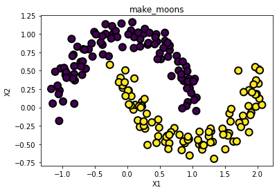
make_moons
- 초승달 모양 데이터 두 집단을 생성
In [ ]:
# 데이터 로딩 및 확인
from sklearn.datasets import make_moons

X, y = make_moons(n_samples = 200, noise = 0.1, random_state= 0 )

print(X[:10])
print(y[:10])
[[ 0.79235735  0.50264857]
 [ 1.63158315 -0.4638967 ]
 [-0.06710927  0.26776706]
 [-1.04412427 -0.18260761]
 [ 1.76704822 -0.19860987]
 [ 1.90607398 -0.07109159]
 [ 0.96219213  0.26198607]
 [ 0.88681385 -0.48489624]
 [ 0.8689352   0.36109278]
 [ 1.15352953 -0.57235293]]
[0 1 1 0 1 1 0 1 0 1]
In [ ]:
# 그림으로 확인[*]
fig = plt.figure()
ax = plt.axes()

ax.scatter(X[:, 0], X[:, 1], marker='o', c=y, s=100,
            edgecolor="k", linewidth=2)

ax.set_xlabel("X1")
ax.set_ylabel("X2")
ax.set_title("make_moons")

plt.show()
make_gaussian_quantiles
- 다변수 정규 분포를 따르는 점들을 생성
In [ ]:
# 데이터 로딩 및 확인[+]
from sklearn.datasets import make_gaussian_quantiles

X, y = make_gaussian_quantiles(n_samples=200, n_features=2, n_classes=2, random_state=0)

print(X[:10])
print(y[:10])
[[-0.34791215  0.15634897]
 [-1.04855297 -1.42001794]
 [-0.39944903  0.37005589]
 [ 0.93184837  0.33996498]
 [-0.87079715 -0.57884966]
 [ 0.15650654  0.23218104]
 [-0.36918184 -0.23937918]
 [-0.49803245  1.92953205]
 [ 1.49448454 -2.06998503]
 [-0.36469354  0.15670386]]
[0 1 0 0 0 0 0 1 1 0]
In [ ]:
# 그림으로 확인
fig = plt.figure()
ax = plt.axes()

ax.scatter(X[:, 0], X[:, 1], marker='o', c=y, s=100,
            edgecolor="k", linewidth=2)

ax.set_xlabel("X1")
ax.set_ylabel("X2")
ax.set_title("make_gaussian_quantiles")

plt.show()

In [ ]: